Oracle Exadata Statistics in AWR report – Part 2 (Outliers)

This blog post is a continuation of the previous blog post titled , Oracle Exadata Statistics in AWR report – Part 1 (Basics). In this post we continue on to describe the performance details displayed in the section “Exadata Outlier Summary”.

Outlier Summary Cell Level

awex3-1

This section displays cells that have performance outliers. The Awr Views DBA_HIST_CELL_DISK_SUMMARY, and DBA_HIST_CELL_GLOBAL_SUMMARY contains samples for each cell, disk and flash card.
The individual sample values, the number of samples, the average, the square of the value are all stored. Using this data the mean and the standard deviation are calculated and the range is defined as the average + or – standard deviation. Cells that have values that are above the mean + standard deviation are displayed.

This section will help us identify cells that have performance metrics, which are outside of the standard operating norms of that cell.

Outlier Summary – Disk Level

awex3-2

This section displays Disks that have performance outliers. The Awr Views DBA_HIST_CELL_DISK_SUMMARY contains this info.The individual sample values, the number of samples, the average, the square of the value are all stored. Using this data the mean and the standard deviation are calculated and the range is defined as the average + or – standard deviation. Disks that have values that are above the mean + standard deviation are displayed.

This section will help us identify Disks (Flash or Hard disk) that have performance metrics, which are outside of the standard operating norms of that Disk.

Exadata OS IO Statistics – Outlier Cells

awex4-1

This section displays cells that have IO statistics that are outliers. Per Cells averages, Per Disk Mean, Standard Deviation, Range’s of the IOPS and IO MBPS information is displayed. Averages exceeding the maximum stated capacity of the disk or cell are shown in Dark red.

This section helps identify whether there are cells or disks that exceed their stated capacities.

Exadata OS IO Statistics – Outlier Disks

awex4-2

This section displays disks (Flash and Hard disk) that have IO statistics that are outliers. Per Disk Mean, Standard Deviation, Range’s of the IOPS, IO MBPS and Disk utilization percentage information is displayed. Averages exceeding the Normal Ranges are shown in Dark red.

This section helps identify whether there are disks that are outside of the standard operating norms of that disk.

Exadata OS IO Latency – Outlier Cells

awex4-3
This section displays cells (Flash and Hard disk) that have IO latencies that are outliers.
Aggregated Across all cells, the Mean, Standard Deviation, Range’s of Average Serice times and Average Wait Times are displayed.
If there are cells Averages that exceed the Normal Range, they are displayed as outliers.

This section helps us identify whether there are cells that have I/O latencies that are outside of the standard operating norms for cells in this system.

Exadata OS IO Latency – Outlier Disks

awex5-1
This section displays disks (Flash and Hard disk) that have IO latencies that are outliers.
Aggregated Across all cells, the Mean, Standard Deviation, Range’s of Average Serice times and Average Wait Times are displayed.
If there are disks whose Averages that exceed the Normal Range of the cells, they are displayed as outliers.

This section helps us identify whether there are disks that have I/O latencies that are outside of the standard operating norms for disks in this system.
Exadata OS CPU Statistics – Outlier Cells

awex5-2
This section displays cells that have Cpu utilization that are outliers.
Aggregated Across all cells, the Mean, Standard Deviation, Range’s of Cpu utilization is displayed.
If there are cells whose Average Cpu utilization that exceed the Normal Cpu utilization Range of the cells, they are displayed as outliers.

Oracle Exadata Statistics in AWR report – Part 1 (Basic Info)

Starting with Exadata storage server 12.1.2.1.0 , used in combination with Oracle Database release 12.1.0.2, there are new sections which have been added to the Oracle AWR (Automatic Worload repository) report, that displays statistics at the Exadata storage level.

This is a really valuable enhancement, which helps with drilling down from database level statistics to cell level statistics, to identify and analyze the workload profile.
You can click on the URL’s in the section “Exadata Configuration and Statistics” to access this part of the report.

There are a few AWR history tables that store this information.

DBA_HIST_CELL_CONFIG
DBA_HIST_CELL_CONFIG_DETAIL
DBA_HIST_CELL_DB
DBA_HIST_CELL_DISKTYPE
DBA_HIST_CELL_DISK_NAME
DBA_HIST_CELL_DISK_SUMMARY
DBA_HIST_CELL_GLOBAL
DBA_HIST_CELL_GLOBAL_SUMMARY
DBA_HIST_CELL_IOREASON
DBA_HIST_CELL_IOREASON_NAME
DBA_HIST_CELL_METRIC_DESC
DBA_HIST_CELL_NAME
DBA_HIST_CELL_OPEN_ALERTS

The description of these views can be found in the Exadata Storage Server Users Guide.

The section starts off by showing the cell configuration information. Then it displays the Kernel  and the Cell Image version’s.

awex1-1

This information comes from the awr view DBA_HIST_CELL_DISK_SUMMARY.

The next section titled “Exadata Storage Information” storage information shows the number of disks and flash cards in each cell and the entire rack.

awex1-2
The first row of the output shows the amount of flash cache in each cell, The size of the smart flash log, Number of hard disks in a cell, Number of flash cards in each cell, and the number of Grid Disks in each cell.
The second row shows the above columns aggregated for all cells in the rack.

The next section titled “Exadata Griddisks” shows the grid disk names, Number of Grid disks in each cell, the Grid Disk size and The type of Drive

awex1-3
The next section titled “Exadata Cell Disks” shows the Disk type, Size of the cell disk, Number of disks .

awex2-1
The next section “ASM disksgroups” shows the diskgroups used by this database.

awex2-2
It shows the diskgroup name,Total size of the diskgroup,Used space, Number of disks in the diskgroup and the redundancy type.

This is followed by a section “Exadata Server Health Report”, which has 3 sub sections Exadata Alerts Summary,Exadata Alerts Detail,Exadata Non-Online Disks which displays information regarding alerts on the cells and any offline disks.
The remaining sections of Exadata performance statistics in the AWR report, display a great deal of Exadata cell performance numbers.

Before we venture much into those sections, it is important to understand some cell level concepts and how they are captured in Awr.

At the cell level if you list the following attributes (On a x5-2 cell with HD drives)

list cell attributes maxpdiops,maxpdmbps,maxfdiops,maxfdmbps you get the following values

167 111 8929 343

These values are collected and stored in the confval column in DBA_HIST_CELL_CONFIG_DETAIL in an XML format.

These base values are used to calculate the maximum capacities of the cells and disks in the sections that follow.

Adaptive Query Optimization – Adaptive Plans – A primer

Based on the available statistics on the objects, the Oracle optimizer could incorrectly estimate the cardinality of certain row sources, resulting in a sub-optimal plan. Adaptive plans are a technique used by the Oracle 12c optimizer to adapt a plan, based on information learned during execution, to pick a better plan.

For eg: If the optimizer estimated the where clause item_id = 20, is going to generate 10 rows and in reality if there were 100,000 rows in the table with item_id = 20, the optimizer might have chosen a nested loops join to this table. With adaptive plans, the optimizer gets the opportunity to switch this nested loops to a hash join, during the execution of this statement.

When the sql statement is parsed, the optimizer creates what is called a “default plan”. If there are some incorrect cardinality estimates performed by the optimizer, then it is probable that it has picked an execution plan with wrong join methods. An adaptive plan, contains multiple pre-determined “Sub plan’s”. A subplan is a portion of the plan that the optimizer can switch to as an alternative at runtime. The optimizer cannot change the whole execution plan at Execution time, it can adapt portions of it.

There are multiple “Statistics Collector’s”, inserted as rowsource’s, at key points in the execution plan.

During execution the statistics collector buffers some rows received by the subplan. Based on the information observed by the collector, the optimizer chooses a specific subplan.

Based on the observations of the statistics collectors a “Final plan” is then chosen by the optimizer and executed. After the first execution, any subsequent execution of this statement, uses this “final plan”. ie it does not incur the overhead of the statistics collection at execution time.

Let us take a look at the following sql statement and its execution plan.

SELECT product_name
FROM order_items o, product_information p
WHERE o.unit_price = 15
AND quantity > 1
AND p.product_id = o.product_id
/

This is a sql where the oracle 12c optimizer, decides to use Adaptive optimization.
If we use dbms_xplan.display_cursor to show the execution plan, it shows the following. This is the “final plan”

SQL_ID  971cdqusn06z9, child number 0                                                                                                                                      
-------------------------------------                                                                                                                                      
SELECT product_name   FROM   order_items o, product_information p                                                                                                          
WHERE  o.unit_price = 15  AND    quantity > 1   AND    p.product_id =                                                                                                      
o.product_id                                                                                                                                                               
                                                                                                                                                                           
Plan hash value: 1553478007                                                                                                                                                
                                                                                                                                                                           
------------------------------------------------------------------------------------------                                                                                 
| Id  | Operation          | Name                | Rows  | Bytes | Cost (%CPU)| Time     |                                                                                 
------------------------------------------------------------------------------------------                                                                                 
|   0 | SELECT STATEMENT   |                     |       |       |     7 (100)|          |                                                                                 
|*  1 |  HASH JOIN         |                     |     4 |   128 |     7   (0)| 00:00:01 |                                                                                 
|*  2 |   TABLE ACCESS FULL| ORDER_ITEMS         |     4 |    48 |     3   (0)| 00:00:01 |                                                                                 
|   3 |   TABLE ACCESS FULL| PRODUCT_INFORMATION |     1 |    20 |     1   (0)| 00:00:01 |                                                                                 
------------------------------------------------------------------------------------------                                                                                 
                                                                                                                                                                           
Outline Data                                                                                                                                                               
-------------                                                                                                                                                              
                                                                                                                                                                           
  /*+                                                                                                                                                                      
      BEGIN_OUTLINE_DATA                                                                                                                                                   
      FULL(@"SEL$1" "P"@"SEL$1")                                                                                                                                           
      USE_HASH(@"SEL$1" "P"@"SEL$1")                                                                                                                                       
      IGNORE_OPTIM_EMBEDDED_HINTS                                                                                                                                          
      OPTIMIZER_FEATURES_ENABLE('12.1.0.2')                                                                                                                                
      DB_VERSION('12.1.0.2')                                                                                                                                               
      ALL_ROWS                                                                                                                                                             
      OUTLINE_LEAF(@"SEL$1")                                                                                                                                               
      FULL(@"SEL$1" "O"@"SEL$1")                                                                                                                                           
      LEADING(@"SEL$1" "O"@"SEL$1" "P"@"SEL$1")                                                                                                                            
      END_OUTLINE_DATA                                                                                                                                                     
  */                                                                                                                                                                       
                                                                                                                                                                           
Predicate Information (identified by operation id):                                                                                                                        
---------------------------------------------------                                                                                                                        
                                                                                                                                                                           
   1 - access("P"."PRODUCT_ID"="O"."PRODUCT_ID")                                                                                                                           
   2 - filter(("O"."UNIT_PRICE"=15 AND "QUANTITY">1))                                                                                                                      
                                                                                                                                                                           
Note                                                                                                                                                                       
-----                                                                                                                                                                      
   - this is an adaptive plan           

Since the Notes section says that this is an adaptive plan, we can use dbms_xplan to show the “full plan”, which includes the “default plan” and the “sub plan’s”
We have to use the ADAPTIVE keyword in dbms_xplan to display the ‘full plan’.

SELECT * FROM TABLE(DBMS_XPLAN.DISPLAY_CURSOR('971cdqusn06z9',0,'ALLSTATS LAST +ADAPTIVE'))

SQL_ID  971cdqusn06z9, child number 0                                                                                                                                      
-------------------------------------                                                                                                                                      
SELECT product_name   FROM   order_items o, product_information p                                                                                                          
WHERE  o.unit_price = 15  AND    quantity > 1   AND    p.product_id =                                                                                                      
o.product_id                                                                                                                                                               
                                                                                                                                                                           
Plan hash value: 1553478007                                                                                                                                                
                                                                                                                                                                           
--------------------------------------------------------------------------------------------------------------------------------------------------------                   
|   Id  | Operation                     | Name                   | Starts | E-Rows | A-Rows |   A-Time   | Buffers | Reads  |  OMem |  1Mem | Used-Mem |                   
--------------------------------------------------------------------------------------------------------------------------------------------------------                   
|     0 | SELECT STATEMENT              |                        |      1 |        |     13 |00:00:00.01 |      24 |     20 |       |       |          |                   
|  *  1 |  HASH JOIN                    |                        |      1 |      4 |     13 |00:00:00.01 |      24 |     20 |  2061K|  2061K|  445K (0)|                   
|-    2 |   NESTED LOOPS                |                        |      1 |      4 |     13 |00:00:00.01 |       7 |      6 |       |       |          |                   
|-    3 |    NESTED LOOPS               |                        |      1 |      4 |     13 |00:00:00.01 |       7 |      6 |       |       |          |                   
|-    4 |     STATISTICS COLLECTOR      |                        |      1 |        |     13 |00:00:00.01 |       7 |      6 |       |       |          |                   
|  *  5 |      TABLE ACCESS FULL        | ORDER_ITEMS            |      1 |      4 |     13 |00:00:00.01 |       7 |      6 |       |       |          |                   
|- *  6 |     INDEX UNIQUE SCAN         | PRODUCT_INFORMATION_PK |      0 |      1 |      0 |00:00:00.01 |       0 |      0 |       |       |          |                   
|-    7 |    TABLE ACCESS BY INDEX ROWID| PRODUCT_INFORMATION    |      0 |      1 |      0 |00:00:00.01 |       0 |      0 |       |       |          |                   
|     8 |   TABLE ACCESS FULL           | PRODUCT_INFORMATION    |      1 |      1 |    288 |00:00:00.01 |      17 |     14 |       |       |          |                   
--------------------------------------------------------------------------------------------------------------------------------------------------------                   
                                                                                                                                                                           
Predicate Information (identified by operation id):                                                                                                                        
---------------------------------------------------                                                                                                                        
                                                                                                                                                                           
   1 - access("P"."PRODUCT_ID"="O"."PRODUCT_ID")                                                                                                                           
   5 - filter(("O"."UNIT_PRICE"=15 AND "QUANTITY">1))                                                                                                                      
   6 - access("P"."PRODUCT_ID"="O"."PRODUCT_ID")                                                                                                                           
                                                                                                                                                                           
Note                                                                                                                                                                       
-----                                                                                                                                                                      
   - this is an adaptive plan (rows marked '-' are inactive)        

In the plan we can see the statistics collector row source. We can see that the Index access “Access Method” was evaluated and discarded by the optimizer. You can see that the optimizer estimated 1 row from product_information and actually it returned 288 rows. The optimizer calcluates an inflection point after which the nested loops operation becomes less efficient and chooses the full scans followed by the hash join.

As indicated in the Note section, the lines that have a – at the beginning of the line, are inactive in the “Final Plan”.

Let us check the flags from v$sql

select is_reoptimizable,is_resolved_adaptive_plan
from v$sql where
sql_id = '971cdqusn06z9'

I I
- -
Y Y

The output indicates that the statement is re-optimizable and that it was resolved by using an adaptive plan.

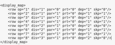
Every step in the ‘full plan’ is stored in v$sql_plan, the information regarding which steps are ‘on’ or ‘off’ in the ‘final plan’ is stored in the column other_xml, under the xml element, display_map.

This is how it looks for sqlid 971cdqusn06z9

xml2

The op= property in the xml, maps to the id column in v$sql_plan (ie the step number). The skp= property indicates whether the step is active in the final plan or not. A value of 1 indicates that, that row is skipped in the final plan. You can display it in a row format with the following sql

select * from
  (SELECT dispmap.*
  FROM v$sql_plan,
    XMLTABLE ( '/other_xml/display_map/row' passing XMLTYPE(other_xml) COLUMNS
      op  NUMBER PATH '@op',    
      dis NUMBER PATH '@dis',   
      par NUMBER PATH '@par',   
      prt NUMBER PATH '@prt',   
      dep NUMBER PATH '@dep',   
      skp NUMBER PATH '@skp' )  
  AS dispmap
  WHERE sql_id     = '&sql_id'
  AND child_number = &sql_child
  AND other_xml   IS NOT NULL
  )
/

      OP        DIS        PAR        PRT        DEP        SKP
---------- ---------- ---------- ---------- ---------- ----------
         1          1          0          0          1          0
         2          1          1          0          1          1
         3          1          1          0          1          1
         4          1          1          0          1          1
         5          2          1          0          2          0
         6          2          1          0          1          1
         7          2          1          0          1          1
         8          3          1          0          2          0

This output can be joined with v$sql_plan to produce an output of the “final plan” .

SELECT
  NVL(map.dis,0) id,
  map.par         parent,
  map.dep         depth,
  lpad(' ',map.dep*1,' ')
  || sp.operation AS operation,
  sp.OPTIONS,
  sp.object#,
  sp.object_name
FROM v$sql_plan sp,
  (SELECT dispmap.*
  FROM v$sql_plan,
    XMLTABLE ( '/other_xml/display_map/row' passing XMLTYPE(other_xml) COLUMNS
      op  NUMBER PATH '@op',
      dis NUMBER PATH '@dis',
      par NUMBER PATH '@par',
      prt NUMBER PATH '@prt',
      dep NUMBER PATH '@dep',
      skp NUMBER PATH '@skp' )
  AS dispmap
  WHERE sql_id     = '&sql_id'
  AND child_number = &sql_child
  AND other_xml   is not null
  ) map
WHERE sp.id             = map.op(+)
AND sp.sql_Id           = '&sql_id'
AND sp.child_number     = &sql_child
AND nvl(map.skp,0)     != 1
ORDER BY nvl(map.dis,0)

If you look at the 10053 trace for the sql, you can see how the optimizer calculates an inflection point.

References

What’s new in 12c

https://martincarstenbach.wordpress.com/2015/01/13/adaptive-plans-and-vsql_plan-and-related-views/

Adaptive Plans Inflection points

Adaptive Dynamic Sampling – Oracle 12c – Some notes

Adaptive Query optimization, was a set of new capabilities, introduced in oracle 12c, to allow the optimizer to discover additional information regarding statistics and make run-time adjustments to execution plans to make them better. This is a major change in the optimizer behaviour from 11g.

I would recommend anyone who is planning an upgrade to 12c, that they make themselves familiar with the following white papers from oracle.

Understanding Optimizer Statistics with Oracle 12c

Best practices for gathering statistics with Oracle 12c

What to expect with the optimizer, with Oracle 12c.

In this article, i want to talk about some of the important concepts behind Dynamic Statistics, which is one of the components of Adaptive query optimizations.

In the section’s that are following, i show some commands to turn some of these features off. I want to be clear that I am not recommending that you turn anything off. I would prefer that customer’s adopt these new features,that are designed to improve the execution plans. Also keep in mind that the following are accurate (Afaik) on 12.1.0.2 as off the time of writing of this article, and are subject to change.

Dynamic statistics has two interesting effects, that DBA’s tend to notice initially.
– Ever so slightly, longer parse times for queries.
– Execution plan changes (Compared to what they had before upgrading) for the same query. (Sometimes unwelcome changes, especially for deployments that value stability more than performance gains).

Dynamic sampling was introduced by oracle in 9i Release 2 to improve the optimizer’s functioning. The amount of dynamic sampling done , and when it kicks in, is controlled by the parameter optimizer_dynamic_sampling. With 12c there is a new concept of Adaptive Dynamic sampling. Adaptive Dynamic Sampling is different from the pre-12c traditional dynamic sampling, in the following aspects.

– Adaptive Dynamic sampling could kick in even when optimizer_dynamic_sampling is set to 2.

– Especially for parallel queries on large tables.

– Adaptive Dynamic sampling kicks in when optimizer_dynamic_sampling is set to 11.
– Adaptive Dynamic sampling issues more queries than dynamic sampling used to do.

– The traditional dynamic sampling, used to issue, atmost, 1 query per table SQL.
– It is not uncommon to see 10’s of Adaptive Dynamic sampling queries being issued for a     single SQL. Multiple dynamic sampling queries for the same table.(It dpends on the volume of data, number of indexed columns, complexity of     the predicates etc).
– If you run a 10046 trace on the query, you will see a lot of additional queries in there that     have the DS_SVC hint in them, which are the queries issued by the Adaptive Dynamic             Sampling.

Setting OPTIMIZER_ADAPTIVE_FEATURES=FALSE does NOT turn off Adaptive Dynamic Sampling.

You can set Optimizer_Dynamic_Sampling = 0 to turn Adaptive Dynamic Sampling off. However this would be like throwing the baby out with the bath water. Setting Optimizer_Dynamic_Sampling=0 completely sets dynamic sampling off (Including the old style pre-12c dynamic sampling).

You can do an ALTER SESSION SET “_fix_control”=’7452863:0′; to turn just Adaptive Dynamic Sampling off, if you so desire.

Adaptive Dynamic Sampling also uses oracle Results Cache. If results cache is enabled in the database (usually by setting result_cache_max_size to a value > 0), then Adaptive dynamic sampling uses the results cache to store the results that it queries up. This is done so that, if there are multiple query parses that have to do dynamic sampling, and they are looking at the same data, the optimizer can just look that value up from the results cache (As opposed to having to query the tables again and again).

If you have a system, that has a lot of hard parses (Due to not using bind variables), you could pottentialy see latch free waits on “Results Cache: rc latch”. Please refer to Mos note 2002089.1, that suggest’s setting “_optimizer_ads_use_result_cache” = FALSE; to work around this. Keep in mind that setting this parameter does not prevent the optimizer from using Adaptive dynamic sampling. All it does it prevent the Adaptive dynamic sampling from using the results cache.

The following Mos note’s and a presentation from Trivadis, have a lot of great information in this regard.

Automatic Dynamic Statistics (Doc ID 2002108.1)

Different Level for Dynamic Statistics (Dynamic Sampling) used than the Level Specified (Doc ID 1102413.1)

High Waits for ‘cursor: pin S wait on X’ due to Dynamic Sampling Against Parallel Queries (Doc ID 2006145.1)

Adaptive Dynamic Sampling – Trivadis

AWR – Profiling Database I/O

Oracle Awr (Automatic Workload Repository) statistics, captures and stores fine grained information about file reads and writes (aka i/o), that the database performed, during the course of execution of, application generated database workloads. When analyzing the read and write patterns of the database, it helps a lot to understand what type of activity is generating the reads and writes. With this stored information we can get an indepth understanding of the distribution of random and sequential reads and writes.

I use this information for getting a better understanding of the I/O profile, for my Exadata sizing exercises.

This information can be used to understand clearly how much of the i/o is from Temp activity, Datafile reads and writes, Archivelog writes, log writes, and whether these are small or large reads and writes.

To the best of my understanding the small reads and writes are those < 128k and the large reads and writes are those > 128k.

This information is contained mainly in two awr Views.

Dba_Hist_Iostat_FileType
Dba_Hist_Iostat_Function

Dba_Hist_Iostat_FileType

This view displays the historical i/o statistics by file type. The main filetypes are the following

Archive Log
Archive Log Backup
Control File
Data File
Data File Backup
Data File Copy
Data File Incremental Backup
Data Pump Dump File
Flashback Log
Log File
Other
Temp File

Dba_Hist_Iostat_Function

This view displays the historical i/o statistics by i/o function. The main i/o functions are the following

Recovery
Buffer Cache Reads
Others
RMAN
Streams AQ
Smart Scan
Data Pump
XDB
Direct Writes
DBWR
LGWR
Direct Reads
Archive Manager
ARCH

From everything i have seen sofar, these reads and writes can be directly co-related to the “Physical read total IO requests” and “Physical write total IO requests” system level statistics.

I have written a script that displays information from the above mentioned views and gives a detailed breakdown of i/o gendrated from different aspects of the database activities.
In order to fit in the computer screen real estate, i have actually limited the columns the script displays (So it displays only the file types i am frequently interested in). Please feel free to take the script and modify it to add columns that you want to display.

The full version of the script  awrioftallpct-pub.sql can be found here.

The script accepts the following inputs
– A begin snap id for a snapid range you want to report for
– A End snap id for a snapid range you want to report for
– A Dbid for the database
– The snap interval in seconds (If you have a 30 minute interval input 1800 seconds)

A description of all the column names in the output, broken down by section, is provided in the header section of the script.

There are 6 sections to this script

1) Total Reads + Writes
2) Total Reads
3) Total Writes
4) Read write breakdown for datafiles
5) Data File – Direct Path v/s Buffered Read Write breakdown
6) Read write breakdown for tempfiles

1) Total Reads + Writes

This section displays the number of reads+writes by filetype, and a percentage of reads+writes for each file type, as a percentage of total reads+writes. The last column displays the total reads+writes for all file types. The column DTDP shows the i/o that bypasses flash cache by default and goes directly to spinning disk on Exadata (Temp+Archivelogs+Flashback Logs).

io1-rw

Click on the image to see a larger version

2) Total Reads

This section displays the number of reads by filetype, and a percentage of reads for each file type, as a percentage of total reads. The last column displays the total reads for all file types.

io1-r

Click on the image to see a larger version

3) Total Writes

This section displays the number of writes by filetype, and a percentage of writes for each file type, as a percentage of total writes. The last column displays the total writes for all file types.

io1-w

Click on the image to see a larger version

4) Read write breakdown for datafiles

This section displays the I/O information only pertaining to datafile i/o. It displays the small and large reads and writes and a percentage they constitute of the total reads+writes to datafiles, and a percentage they constitute of the total reads or writes to datafiles. It also displays the total small and large reads and writes and a percentage they constitute of the total reads+writes to datafiles.

io1-dfrw

Click on the image to see a larger version

5) Data File – Direct Path v/s Buffered Read Write breakdown

This section provides a breakdown of I/O by function (As opposed to i/o by filetype in the previous sections). The output shows columns that display the direct path small and large reads and writes, buffered small reads and writes, smart scan small and large reads and other small and large reads and writes.

io3-bf

Click on the image to see a larger version

6) Read write breakdown for tempfiles

This section displays the I/O information only pertaining to tempfile i/o. It displays the small and large reads and writes and a percentage they constitute of the total reads+writes to tempfiles, and a percentage they constitute of the total reads or writes to tempfiles. It also displays the total small and large reads and writes and a percentage they constitute of the total reads+writes to tempfiles.

io3-tf

Click on the image to see a larger version

The full version of the script  awrioftallpct-pub.sql can be found here.

Oracle Active DataGuard – Considerations for the Wide area Network

Oracle customers use Oracle Active Dataguard to create and maintain one or many standby databases that protect their mission critical primary databases from disaster. Typically, in such deployments, the primary databases and standby databases are in geographically separate locations connected via a WAN (Wide Area Network). Log Transport Services, transfers Large volumes of redo logs from the primary location to the standby, using Sql*Net.

We have to ensure that all the components from the source to target are setup correctly to ensure that the data transfer can be done with the best throughput possible. If sufficient network bandwidth is not available with reasonable latencies, then we will start seeing the log transfer and apply,lagging on the standby site (Which is oracle speak for, your primary and standby database is now out of sync from a data perspective).

One key point to keep in mind is that, lower the network round trip time (aka latency), higher your data transfer throughput. Higher the network round trip time (aka latency), lower your data transfer throughput. So it is very important to maintain low round trip times on your Wide area network.

To understand network data transfer throughput, It is important to understand the the concepts of Tcp Window Size and Bandwidth Delay Product (aka BDP).

Tcp Window size is the amount of bytes that can be transmitted without receiving an acknowledgement from the other side. Once Tcp Window size amount of bytes are send, the sender stops sending any more bytes and waits for an acknowledgement from the receiver.

Bandwidth delay product is calculated as the product of the network bandwidth and network round trip time. bdp=network bandwidth*round trip time. This is the amount of data that left the sender before the first acknowledgement was received by the sender. If the senders output bandwidth is stable, and the bandwidth is fully used, then the BDP calculates the number of packets in transit. If we set the Tcp Window size equal to the bandwidth delay product, then in theory we should be able to fully utilize the available bandwidth.

Setup the network

We have to start by setting up the networking components to support the desired/stated bandwidth. So if you have a WAN that is a 10GigE network, all the NIC’s (Network interface cards), ports, switches in the configuration should be configured to support 10GigE full Duplex settings. After setup, run the configuration display utilities and ensure that all these component levels the transfer speeds are set to be 10 GigE. Customers often run into trouble when Auto Negotiation causes some NIC’s to set the transfer speeds to 1GigE because of configuration mismatches.

Use tools like Iperf to test the transfer speeds that your network is capable of achieving.

One important aspect to keep in mind is that it is probable that the WAN is shared by other traffic (e-mail, data replication, san replication). This has two important implications that we should consider.

  • If there is a lot of bandwidth consumption by some of this miscellaneous traffic, round trip times could be degraded periodically on the network.
  • We should be careful in our calculations that we do not completely consume the entire bandwidth for redo transport. (This could impact other processes)
    • So it is important to figure out (Working with the network admins) what the bandwidth entitlements are for redo transport and base our calculations on those numbers.

Caclulate our BDP

Use the following formula to calculate our Bandwidth delay product (BDP)

(bandwidth/8)*rount trip time in seconds.

The network bandwidth is expressed in bits per second, so we divide by 8 to convert to bytes.
Round Trip Time is usually in milli seconds, so we divide by 1000 to convert to seconds.

So for example, if we have a 10Gbit network bandwidth and a 40ms round trip time

BDP=(10000000000/8)*(40/1000) = 50,000,000 bytes.

Setup Sql*Net Parameters

The current recommendations for Dataguard Redo transport are as follows.

Set the SDU size to 65535

  • We can set SDU on a per connection basis using the SDU parameter in the local naming configuration file (TNSNAMES.ORA) and the listener configuration file (LISTENER.ORA)
  • We can set the SDU for all Oracle Net connections with the profile parameter DEFAULT_SDU_SIZE in the SQLNET.ORA file.

Set TCP.NODELAY to YES

To preempt delays in buffer flushing in the TCP protocol stack, disable the TCP Nagle algorithm by setting TCP.NODELAY to YES in the SQLNET.ORA file on both the primary and standby systems.

Setup RECV_BUF_SIZE and SEND_BUF_SIZE

The current recommendation is to set the SEND_BUF_SIZE and RECV_BUF_SIZE parameters (Which are the send and receive socket buffer sizes for SQL*Net) to 3 Times the BDP.

As per the above example we would set them to 50,000,000*3 = 150,000,000

Setup Operating system Kernel Parameters

If you are using the Linux operating system make sure that the values for the following kernel parameters are setup to be higher than the values set for RECV_BUF_SIZE and SEND_BUF_SIZE.

net.core.rmem_max
net.core.wmem_max

Once we have configured the network, operating system and the sql*net, and we have redo transfer, we can perform further network monitoring to see how the network bandwidth is being utilized, and make appropriate adjustments.

Links to helpful Documents

Iperf

How to calcluate Tcp throughput for long distance links (blog)

Oracle Net Performance Tuning (Mos)

Setting Send and Receive Buffer Sizes (Mos)

Tuning Sql*Net peformance (Oracle Docs)

Configuring Oracle Dataguard (Oracle Docs)

Best Practices for Sync Data Transport (White Paper)

Script to compare tkprof output files

I often use the oracle 10046 event tracing mechanism to capture sql’s from a session to identify why certain transactions are running slower in different env’s or at different points in time. Oracle does have a mechanism where you can save the trace information in database tables. One can use the INSERT parameter in tkprof to store the trace information into a database table. Once in the table you can write sql’s that compare multiple runs or multiple statements.

I wrote a python program that compares two different tkprof output files. The files are compared, and the following aspects of each of the sqlid’s in the tkprof output file,s are printed side by side. The output is sorted by the Difference in Elapsed Time, in Descending order.

  • Sql text
  • Plan Hash Value
  • Total Elapsed time
  • Total Logical Reads
  • Total Rows processed
  • Difference in Elapsed Time
  • Difference in Number of Rows processed
  • Difference in Logical reads.

Other columns can be added to this, if you desire.
I use this script output as a quick way to see which sql’s are running slower and are probably candidates for further analysis/tuning.

The sqlid’s from the file provided as the first argument to the script (referred to as the left file) are compared to the same sqlid’s in the file provided as the second argument to the script (referred to as the right file). The following columns are displayed.

sqlid                           sqlid being compared
text                             First 20 chars of the sql text
lplan                           Plan hash value from the left file
rplan                          Plan hash value from the right file
lela                             Total Elapsed time from the left file
rela                            Total Elapsed time from the right file
llreads                       Total Logical reads (query+current) from the left file
rlreads                      Total Logical reads (query+current) from the right file
lrows                         Total rows processed from the left file
rrows                        Total rows processed from the right file
eladiff                        Lela – Rela
rowsdiff                    Lrows – Rrows
lreadsdiff                  Llreads – rlreads

Here is a sample syntax for running the script. (You need the python pandas package to be installed for this to execute successfully)

python ./difftk.py /u01/tkprofout/Newplans.prf /u01/tkprofout/Stage.prf

Here is a sample output

difftk

Click on the image to view a larger version.

The full script is below

#Python script to list differences between sql executions in two tkprof output files
#useful if comparing tkprof from prod and dev for example
#Author : rajeev.ramdas

import sys
import os
import pandas as pd
from pandas import DataFrame

# Define a class to hold the counters for each sqlid
class sqliddet:
     def init(self):
            sqlid=''
            text=''
            plan_hash=''
            tcount=0
            tcpu=0
            tela=0
            tdisk=0
            tquery=0
            tcurr=0
            trows=0

# Define 2 empty dictionaries to store info about each input file
leftsqliddict={}
rightsqliddict={}

# Process each file and add one row per sqlid to the dictionary
# We want to add the row to the dictionary only after the SQLID row and the total row has been read
# So the firstsqlid flag is used to make sure that we do not insert before total is read for the first row.

def processfile(p_file,p_sqliddict):

    myfile=open(p_file,"r")
    line=myfile.readline()
    firstsqlid=True
    linespastsqlid=99
    while line:
        linespastsqlid+=1
        line=myfile.readline()
        if line.startswith('SQL ID'):
            linespastsqlid=0
            if firstsqlid==True:
                firstsqlid=False
            else:
                p_sqliddict[currsqlid.sqlid]=[currsqlid.plan_hash,currsqlid.tcount,currsqlid.tcpu,currsqlid.tela,currsqlid.tdisk,currsqlid.tquery
                            ,currsqlid.tcurr,currsqlid.trows,currsqlid.text]
            currsqlid=sqliddet()
            currsqlid.sqlid=line.split()[2]
            currsqlid.plan_hash=line.split()[5]
        if linespastsqlid==2:
            currsqlid.text=line[0:20]
        if line.startswith('total'):
            a,currsqlid.tcount,currsqlid.tcpu,currsqlid.tela,currsqlid.tdisk,currsqlid.tquery,currsqlid.tcurr,currsqlid.trows=line.split()
        if line.startswith('OVERALL'):
            p_sqliddict[currsqlid.sqlid]=[currsqlid.plan_hash,currsqlid.tcount,currsqlid.tcpu,currsqlid.tela,currsqlid.tdisk,currsqlid.tquery
                       ,currsqlid.tcurr,currsqlid.trows,currsqlid.text]
        continue
    myfile.close()

# Main portion of script
if len(sys.argv) != 3:
   print('Syntax : python ./difftk.py tkprof1.out tkprof2.out')
   sys.exit()

if not os.path.isfile(sys.argv[1]) or not os.path.isfile(sys.argv[2]):
   print ("File Does not Exist")
   sys.exit()

processfile(sys.argv[1],leftsqliddict)
processfile(sys.argv[2],rightsqliddict)

t_difftk_lst=[]

# Match the sqlid's from the file on the left to the file on the right
# Gather up the statistics form both sides, insert into a list
# Transfer the list to a pandas dataframe, add some computed columns

for sqlid,stats in leftsqliddict.items():
    l_totlogical=int(stats[5])+int(stats[6])
    if sqlid in rightsqliddict:
       t_difftk_lst.append([sqlid,stats[8].rstrip(),stats[0],rightsqliddict[sqlid][0],float(stats[3])
                            ,float(rightsqliddict[sqlid][3]),float(l_totlogical),float(rightsqliddict[sqlid][5])+float(rightsqliddict[sqlid][6])
                            ,float(stats[7]),float(rightsqliddict[sqlid][7])
                           ])
    else:
       t_difftk_lst.append([sqlid,stats[8].rstrip(),stats[0],0,float(stats[3]),0
                            ,float(l_totlogical),0,float(stats[7]),0
                           ])

difftk_df=DataFrame(t_difftk_lst,columns=['sqlid','sqltext','lplan','rplan','lela','rela','llreads','rlreads','lrows','rrows'])
difftk_df['eladiff']=difftk_df['lela']-difftk_df['rela']
difftk_df['rowsdiff']=difftk_df['lrows']-difftk_df['rrows']
difftk_df['lreadsdiff']=difftk_df['llreads']-difftk_df['rlreads']

pd.set_option('display.width',1000)
print (difftk_df.sort(columns='eladiff',ascending=False))

Oracle Database In-Memory an introduction Part 2 – What do i need to do, to use the Oracle In-Memory Database ?

Step 1) Define the INMEMORY_SIZE

Customer has to setup the correct value for a database initialization parameter , INMEMORY_SIZE. This parameter specifies the amount of memory, from the SGA, that is to be used for the In-Memory column store. This is a static pool (ie Automatic memory management cannot extend or shrink this area), which means that you have to restart the database if any changes to this parameter needs to take effect. The In-Memory area is sub-divided into two pools: a 1MB pool used to store the actual column formatted data populated into memory, and a 64K pool used to store metadata about the objects that are populated into the IM column store.


sho parameter inmemory_size

NAME				     TYPE	 VALUE
------------------------------------ ----------- ------------------------------
inmemory_size			     big integer 500M

select pool,alloc_bytes,used_bytes,populate_status from v$inmemory_area;

POOL			   ALLOC_BYTES USED_BYTES POPULATE_STATUS
-------------------------- ----------- ---------- --------------------------
1MB POOL		     418381824		0 DONE
64KB POOL		     100663296		0 DONE

Step 2) Mark the performance critical objects in your database, with the attribute INMEMORY

select partition_name,bytes/(1024),inmemory,inmemory_compression from dba_segments where
owner = 'SH' and segment_name = 'SALES'

PARTITION_NAME		       BYTES/(1024) INMEMORY INMEMORY_COMPRESS
------------------------------ ------------ -------- -----------------
SALES_Q1_1998			       8192 DISABLED

ALTER TABLE SH.SALES MODIFY PARTITION SALES_Q1_1998 INMEMORY PRIORITY CRITICAL MEMCOMPRESS FOR QUERY HIGH;

Table altered.

select partition_name,bytes/(1024),inmemory,inmemory_compression from dba_segments where
owner = 'SH' and segment_name = 'SALES'  2  ;

PARTITION_NAME		       BYTES/(1024) INMEMORY INMEMORY_COMPRESS
------------------------------ ------------ -------- -----------------
SALES_Q1_1998			       8192 ENABLED  FOR QUERY HIGH


Step 3) Populate the In-Memory datastore

Objects are populated into the In-Memory Datastore, in a prioritized list, immediately after the database is opened, or after they are scanned for the first time. There are 7 levels for the keyword PRIORITY (CRITICAL, HIGH, MEDIUM, LOW, NONE).

The IM column store is populated by a set of background processes referred to as worker processes (ora_w001_orcl). The database is fully active / accessible while this occurs.Each worker process is given a subset of database blocks from the object to populate into the IM column store. Population is a streaming mechanism, simultaneously columnizing and compressing the data. There is a new IMCO (In memory co-ordinator) background process which wakes up every 2 minutes and checks to see if there are any population tasks that need to be completed. Eg: A new object has been marked as InMemory with a PRIORITY other than None.

select v.owner,v.segment_name,v.partition_name,v.bytes orig_size,v.inmemory_size in_mem_size

OWNER	   SEGMENT_NA PARTITION_NAME		      ORIG_SIZE IN_MEM_SIZE
---------- ---------- ------------------------------ ---------- -----------
SH	   SALES      SALES_Q1_1998			8388608     1179648

select * from 
(
select /*+ full(sales) */ channel_id,count(*)
from sh.sales partition (sales_q1_1998)
group by channel_id
order by count(*) desc
)
where rownum < 6

CHANNEL_ID   COUNT(*)
---------- ----------
	 3	32796
	 2	 6602
	 4	 3926
	 9	  363

Elapsed: 00:00:00.09

select * from table (dbms_xplan.display_cursor());

PLAN_TABLE_OUTPUT
--------------------------------------------------------------------------------------------------------
SQL_ID	40pjk921r3jrc, child number 0
-------------------------------------
select * from ( select /*+ full(sales) */ channel_id,count(*) from
sh.sales partition (sales_q1_1998) group by channel_id order by
count(*) desc ) where rownum < 6

Plan hash value: 2962696457

---------------------------------------------------------------------------------------------------------
| Id  | Operation			| Name	| Rows	| Bytes | Cost (%CPU)| Time	| Pstart| Pstop |
---------------------------------------------------------------------------------------------------------

PLAN_TABLE_OUTPUT
---------------------------------------------------------------------------------------------------------
|   0 | SELECT STATEMENT		|	|	|	|    12 (100)|		|	|	|
|*  1 |  COUNT STOPKEY			|	|	|	|	     |		|	|	|
|   2 |   VIEW				|	|     4 |   104 |    12  (34)| 00:00:01 |	|	|
|*  3 |    SORT ORDER BY STOPKEY	|	|     4 |    12 |    12  (34)| 00:00:01 |	|	|
|   4 |     HASH GROUP BY		|	|     4 |    12 |    12  (34)| 00:00:01 |	|	|
|   5 |      PARTITION RANGE SINGLE	|	| 43687 |   127K|     9  (12)| 00:00:01 |     5 |     5 |
|   6 |       TABLE ACCESS INMEMORY FULL| SALES | 43687 |   127K|     9  (12)| 00:00:01 |     5 |     5 |
---------------------------------------------------------------------------------------------------------

For much more in-depth technical details of the Oracle Database In-Memory, please see this whitepaper.

Oracle Database In-Memory an introduction Part 1 – What is Oracle Database In-Memory, and how is it different ?

On July 22nd 2014, Oracle corporation, announced Oracle Database 12c’s latest patch release 12.1.0.2. This latest patch release includes the new Oracle Database In-Memory functionality.
The Oracle Database In-Memory enables a single database to efficiently support mixed workloads. It uses a “dual-format” architecture, that retains the Record-Setting OLTP performance of the oracle databases, while simultaneously supporting real-time analytics and reporting. This is achieved by retaining the traditional oracle memory architecture, but adding a new purely in-memory column format (Automatically created and maintained by oracle), optimized for analytical processing.

So now you have the data stored in the Oracle database in your database files, in a row format, and for any of the objects marked as INMEMORY, oracle creates an In-Memory column store, where the data resides in a column format.The IM column store does not replace the buffer cache, but acts as a supplement, so that data can now be stored in memory in both a row and a column format.

Ok why the dual format, one would ask ?

The Row format is retained as is, so that there is no compromise/degradation in the OLTP performance of the database. In a Row format database each row is made up of multiple columns, with each column representing an attribute about that record. A column format database stores each of the attributes about the transaction in a separate column structure. A column format is ideal for Analytics, but is not very efficient in processing DML requests like insert, update and deletes (Which operates on the whole row). Oracle Database In-Memory (Database In-Memory) provides the best of both worlds by allowing data to be simultaneously populated in both an in-memory row format (the buffer cache) and a new in-memory column format (The In-Memory Store).

cncpt_vm_379

The picture above shows the In-Memory area in the SGA

cncpt_vm_378

The above picture shows an example of the Column Store.

No changes are necessary to your existing applications in order to take advantage of the Oracle Database In-Memory option. Any query that will benefit from the In-Memory column store will be automatically directed there, by the Optimizer. The In-Memory store is kept transactionally consistent with the buffer cache. There are numerous optimizations that have been implemented that speed up this data access in the In-Memory store. All the database functionality that Oracle has built over the last 30 years, continues to work in this new version.

It is normal that folks would go out and compare, Oracle Databaes In-Memory, with other In Memory Database products available in the Market today. So let us explore the differences with some of those products next.

TimesTen

Oracle TimesTen In-Memory Database is a,row oriented, memory optimized relational database, that resides entirely in the physical memory of a server. Oracle TimesTen In-Memory Database operates on databases that fit entirely in physical memory using standard SQL interfaces. In contrast, the Oracle Database In-Memory, only stores selected objects, in memory, in a column format (As opposed to a row format in Oracle TimesTen), the remaining objects continue to exist on the storage subsystem.

SAP HANA

SAP HANA is an in-memory, column-oriented relational database. So the entire database has to reside in physical memory of the server. As mentioned earlier in this article, OLTP transactions have some disadvantages while operating on column stores.

Todays databases can be in the 10’s or 100’s of TeraBytes. Storing this entire data in physical memory can be an expensive proposition, not to mention that, it is quite prevalent that ,only a small subset of this data, ends up having daily usage. This is where Oracle’s approach of storing only selected objects in memory, has significant benefits.

Here is a link to the Oracle Database In-Memory Launch.

OraChk Collection Manager

OraChk (Previously known as Raccheck) is a utility from oracle to perform configuration checks on Oracle database platforms, and report on configurations that do not match oracle’s best practices. OraChk has the ability to upload the results of its checks into an oracle database. Details about this utility can be found in Mos Note 1268927.1

Oracle has now released  OraChk Collection Manager which is a companion application to OraChk, which has an Oracle Application Express, Front End which can be used  as a dashboard, in which customers can track their ORAchk, RACcheck and Exachk collection data in one easy to use interface.

Details about downloading and using “OraChk Collection Manager” can be found in Mos Note 1602329.1