Oracle Awr (Automatic Workload Repository) statistics, captures and stores fine grained information about file reads and writes (aka i/o), that the database performed, during the course of execution of, application generated database workloads. When analyzing the read and write patterns of the database, it helps a lot to understand what type of activity is generating the reads and writes. With this stored information we can get an indepth understanding of the distribution of random and sequential reads and writes.
I use this information for getting a better understanding of the I/O profile, for my Exadata sizing exercises.
This information can be used to understand clearly how much of the i/o is from Temp activity, Datafile reads and writes, Archivelog writes, log writes, and whether these are small or large reads and writes.
To the best of my understanding the small reads and writes are those < 128k and the large reads and writes are those > 128k.
This information is contained mainly in two awr Views.
Dba_Hist_Iostat_FileType
Dba_Hist_Iostat_Function
Dba_Hist_Iostat_FileType
This view displays the historical i/o statistics by file type. The main filetypes are the following
Archive Log
Archive Log Backup
Control File
Data File
Data File Backup
Data File Copy
Data File Incremental Backup
Data Pump Dump File
Flashback Log
Log File
Other
Temp File
Dba_Hist_Iostat_Function
This view displays the historical i/o statistics by i/o function. The main i/o functions are the following
Recovery
Buffer Cache Reads
Others
RMAN
Streams AQ
Smart Scan
Data Pump
XDB
Direct Writes
DBWR
LGWR
Direct Reads
Archive Manager
ARCH
From everything i have seen sofar, these reads and writes can be directly co-related to the “Physical read total IO requests” and “Physical write total IO requests” system level statistics.
I have written a script that displays information from the above mentioned views and gives a detailed breakdown of i/o gendrated from different aspects of the database activities.
In order to fit in the computer screen real estate, i have actually limited the columns the script displays (So it displays only the file types i am frequently interested in). Please feel free to take the script and modify it to add columns that you want to display.
The full version of the script awrioftallpct-pub.sql can be found here.
The script accepts the following inputs
– A begin snap id for a snapid range you want to report for
– A End snap id for a snapid range you want to report for
– A Dbid for the database
– The snap interval in seconds (If you have a 30 minute interval input 1800 seconds)
A description of all the column names in the output, broken down by section, is provided in the header section of the script.
There are 6 sections to this script
1) Total Reads + Writes
2) Total Reads
3) Total Writes
4) Read write breakdown for datafiles
5) Data File – Direct Path v/s Buffered Read Write breakdown
6) Read write breakdown for tempfiles
1) Total Reads + Writes
This section displays the number of reads+writes by filetype, and a percentage of reads+writes for each file type, as a percentage of total reads+writes. The last column displays the total reads+writes for all file types. The column DTDP shows the i/o that bypasses flash cache by default and goes directly to spinning disk on Exadata (Temp+Archivelogs+Flashback Logs).

Click on the image to see a larger version
2) Total Reads
This section displays the number of reads by filetype, and a percentage of reads for each file type, as a percentage of total reads. The last column displays the total reads for all file types.

Click on the image to see a larger version
3) Total Writes
This section displays the number of writes by filetype, and a percentage of writes for each file type, as a percentage of total writes. The last column displays the total writes for all file types.

Click on the image to see a larger version
4) Read write breakdown for datafiles
This section displays the I/O information only pertaining to datafile i/o. It displays the small and large reads and writes and a percentage they constitute of the total reads+writes to datafiles, and a percentage they constitute of the total reads or writes to datafiles. It also displays the total small and large reads and writes and a percentage they constitute of the total reads+writes to datafiles.

Click on the image to see a larger version
5) Data File – Direct Path v/s Buffered Read Write breakdown
This section provides a breakdown of I/O by function (As opposed to i/o by filetype in the previous sections). The output shows columns that display the direct path small and large reads and writes, buffered small reads and writes, smart scan small and large reads and other small and large reads and writes.

Click on the image to see a larger version
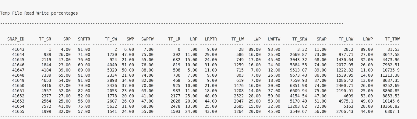
6) Read write breakdown for tempfiles
This section displays the I/O information only pertaining to tempfile i/o. It displays the small and large reads and writes and a percentage they constitute of the total reads+writes to tempfiles, and a percentage they constitute of the total reads or writes to tempfiles. It also displays the total small and large reads and writes and a percentage they constitute of the total reads+writes to tempfiles.

Click on the image to see a larger version
The full version of the script awrioftallpct-pub.sql can be found here.